Chapter 2 Import

2.1 Introduction

The first step in the typical data science project involves importing data into R. There are numerous packages for different data types all with varying preferences on speed and efficiency. Here are some R packages for importing data into R:

2.2 Tabular Data

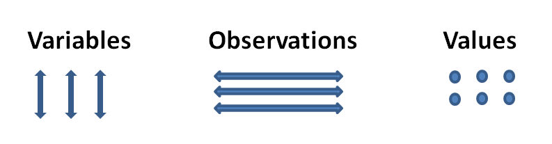
Tabular data consists of variables, observations and values to form data frames. This is the most common format of organized data and many packages are developed to work with this type of data.

2.2.1 readr

readr: Read flat/tabular text files from disk (or a connection). readr has some benefits over the base/utils version as smart column type parsing and not automatically converting strings into factors.

2.2.1.1 Examples

Here is an example of credit card applications data set from the UCI Machine Learning Repository using readr:

library(readr)
cc_apps <- read_csv("http://archive.ics.uci.edu/ml/machine-learning-databases/credit-screening/crx.data", col_names = F)
head(cc_apps)

## # A tibble: 6 × 16
##      X1    X2    X3    X4    X5    X6    X7    X8    X9   X10   X11   X12
##   <chr> <dbl> <dbl> <chr> <chr> <chr> <chr> <dbl> <chr> <chr> <chr> <chr>
## 1     b 30.83 0.000     u     g     w     v  1.25     t     t    01     f
## 2     a 58.67 4.460     u     g     q     h  3.04     t     t    06     f
## 3     a 24.50 0.500     u     g     q     h  1.50     t     f     0     f
## 4     b 27.83 1.540     u     g     w     v  3.75     t     t    05     t
## 5     b 20.17 5.625     u     g     w     v  1.71     t     f     0     f
## 6     b 32.08 4.000     u     g     m     v  2.50     t     f     0     t
## # ... with 4 more variables: X13 <chr>, X14 <chr>, X15 <int>, X16 <chr>

2.2.2 readxl

readxl: Import excel files into R. Supports ‘.xls’ via the embedded ‘libxls’ C library (http://sourceforge.net/projects/libxls/) and ‘.xlsx’ via the embedded ‘RapidXML’ C++ library (http://rapidxml.sourceforge.net). Works on Windows, Mac and Linux without external dependencies.

2.2.2.1 Examples

Here is an example from the default of credit card clients data set from the UCI Machine Learning Repository using readxl:

# download the excel file first from the link
library(readxl)
default_cc <- read_excel("default of credit card clients.xls")

# alternative reading from a URL
require(RCurl)
require(gdata)
url <- "http://archive.ics.uci.edu/ml/machine-learning-databases/00350/default%20of%20credit%20card%20clients.xls"
default_cc <- read.xls(url)

head(default_cc)

##    X        X1  X2        X3       X4  X5    X6    X7    X8    X9   X10
## 1 ID LIMIT_BAL SEX EDUCATION MARRIAGE AGE PAY_0 PAY_2 PAY_3 PAY_4 PAY_5
## 2  1     20000   2         2        1  24     2     2    -1    -1    -2
## 3  2    120000   2         2        2  26    -1     2     0     0     0
## 4  3     90000   2         2        2  34     0     0     0     0     0
## 5  4     50000   2         2        1  37     0     0     0     0     0
## 6  5     50000   1         2        1  57    -1     0    -1     0     0
##     X11       X12       X13       X14       X15       X16       X17
## 1 PAY_6 BILL_AMT1 BILL_AMT2 BILL_AMT3 BILL_AMT4 BILL_AMT5 BILL_AMT6
## 2    -2      3913      3102       689         0         0         0
## 3     2      2682      1725      2682      3272      3455      3261
## 4     0     29239     14027     13559     14331     14948     15549
## 5     0     46990     48233     49291     28314     28959     29547
## 6     0      8617      5670     35835     20940     19146     19131
##        X18      X19      X20      X21      X22      X23
## 1 PAY_AMT1 PAY_AMT2 PAY_AMT3 PAY_AMT4 PAY_AMT5 PAY_AMT6
## 2        0      689        0        0        0        0
## 3        0     1000     1000     1000        0     2000
## 4     1518     1500     1000     1000     1000     5000
## 5     2000     2019     1200     1100     1069     1000
## 6     2000    36681    10000     9000      689      679
##                            Y
## 1 default payment next month
## 2                          1
## 3                          1
## 4                          0
## 5                          0
## 6                          0

2.3 Hierarchical Data

Hierarchical Data is a tree-structure data format such as XML, HTML, JSON. Popular methods for accessing this data are known as web scraping or web data mining when the goal is to parse data on a web page into a analysis-ready format such as a data frame.

2.3.1 jsonlite

jsonlite: A fast JSON parser and generator optimized for statistical data and the web.

2.3.1.1 Examples

TBD

2.3.2 xml2

xml2: Work with XML files using a simple, consistent interface. Built on top of the ‘libxml2’ C library.

2.3.2.1 Examples

TBD

2.3.3 rvest

rvest: Wrappers around the ‘xml2’ and ‘httr’ packages to make it easy to download, then manipulate, HTML and XML.

2.3.3.1 Examples

TBD

2.4 Relational Data

Relational Data consists of a collection of data items (tables) organized as a set based on the data contents and its relation.

2.4.1 DBI

DBI: A database interface definition for communication between R and relational database management systems. All classes in this package are virtual and need to be extended by the various R/DBMS implementations.

2.4.1.1 Examples

TBD

2.4.2 RMySQL

RMySQL: Implements ‘DBI’ Interface to ‘MySQL’ and ‘MariaDB’ Databases.

2.4.2.1 Examples

TBD

2.4.2.2 RPostgreSQL

RPostgreSQL:Database interface and PostgreSQL driver for R This package provides a Database Interface (DBI) compliant driver for R to access PostgreSQL database systems. In order to build and install this package from source, PostgreSQL itself must be present your system to provide PostgreSQL functionality via its libraries and header files. These files are provided as postgresql-devel package under some Linux distributions. On Microsoft Windows system the attached libpq library source will be used. A wiki and issue tracking system for the package are available at Google Code at https://code.google.com/p/rpostgresql/

2.4.2.3 Examples

TBD

2.5 Distributed Data

Distributed Data consists of non-relational formats with quick access to data over a large number of nodes (data spread over many different computers).

2.5.1 sparklyr

sparklyr: Filter and aggregate Spark datasets then bring them into R for analysis and visualization.

2.5.1.1 Examples

TBD

2.6 Additional Import Methods

Different Data Formats: The R programming language and environment is continuously increasing its capacity with new packages to work with different types of proprietory data formats from statistical software packages that are used on industry teams.

2.6.1 haven

haven: Import and Export ‘SPSS’, ‘Stata’ and ‘SAS’ Files.

2.6.1.1 Examples

Here is an example from Macquarie University data repository for the applied finance and actuarial studies of importing a SAS data set:

library(haven)
claims <- read_sas("http://www.businessandeconomics.mq.edu.au/our_departments/Applied_Finance_and_Actuarial_Studies/acst_docs/glms_for_insurance_data/data/claims_sas_miner.sas7bdat")
head(claims)

## # A tibble: 6 × 33
##          ID KIDSDRIV   PLCYDATE TRAVTIME    CAR_USE POLICYNO BLUEBOOK
##       <chr>    <dbl>     <date>    <dbl>      <chr>    <dbl>    <dbl>
## 1 100058542        0 1996-03-17 17.09181    Private 36292520     9860
## 2 100093408        0 1993-07-26 17.98656    Private 31958061     1500
## 3 100208113        0 1994-06-06 47.00727 Commercial 42433312    30460
## 4 100237269        0 1999-01-19 31.24381    Private 49896544    16580
## 5  10042968        0 1999-05-18 13.96243 Commercial 79298192    23030
## 6 100737644        0 1996-02-28 45.79204    Private 43393435    20730
## # ... with 26 more variables: INITDATE <date>, RETAINED <dbl>,
## #   NPOLICY <dbl>, CAR_TYPE <chr>, RED_CAR <chr>, OLDCLAIM <dbl>,
## #   CLM_FREQ <dbl>, REVOLKED <chr>, MVR_PTS <dbl>, CLM_AMT <dbl>,
## #   CLM_DATE <date>, CLM_FLAG <chr>, BIRTH <date>, AGE <dbl>,
## #   HOMEKIDS <dbl>, YOJ <dbl>, INCOME <dbl>, GENDER <chr>, MARRIED <chr>,
## #   PARENT1 <chr>, JOBCLASS <chr>, MAX_EDUC <chr>, HOME_VAL <dbl>,
## #   SAMEHOME <dbl>, DENSITY <chr>, YEARQTR <chr>

2.6.2 foreign

foreign: Functions for reading and writing data stored by some versions of Epi Info, Minitab, S, SAS, SPSS, Stata, Systat and Weka and for reading and writing some dBase files.

2.6.2.1 Examples

TBD

2.6.3 Zipped Data

Accessing Zipped Data files: Zip archives are actually more a ‘filesystem’ with content, meta data, and/or documentation.

Create a temp file. file name (eg tempfile())
Use download.file() to download the file into the temp object that is being reserved for the file
Use unzip() to extract the target file from temp file by reading the meta data on what specific data set you want which is contained in the zip file
Remove the temp file via unlink()

temp <- tempfile()
download.file("http://archive.ics.uci.edu/ml/machine-learning-databases/00222/bank.zip",temp)
unzip(temp, "bank.csv")
bank_marketing <- read.csv("bank.csv", sep=";") # sometimes its the default
unlink(temp)
head(bank_marketing)

##   age         job marital education default balance housing loan  contact
## 1  30  unemployed married   primary      no    1787      no   no cellular
## 2  33    services married secondary      no    4789     yes  yes cellular
## 3  35  management  single  tertiary      no    1350     yes   no cellular
## 4  30  management married  tertiary      no    1476     yes  yes  unknown
## 5  59 blue-collar married secondary      no       0     yes   no  unknown
## 6  35  management  single  tertiary      no     747      no   no cellular
##   day month duration campaign pdays previous poutcome  y
## 1  19   oct       79        1    -1        0  unknown no
## 2  11   may      220        1   339        4  failure no
## 3  16   apr      185        1   330        1  failure no
## 4   3   jun      199        4    -1        0  unknown no
## 5   5   may      226        1    -1        0  unknown no
## 6  23   feb      141        2   176        3  failure no